The Elephant in the corner of the room (and other thoughts on dating the Pleistocene extinctions)

Telling time is important to scientists who work in the deep past. As humans, we find it difficult to tell time beyond the scale of a lifetime. Last week runs into last month. Those months build up into years and decades. To those of us born in the 1970s, 25 years ago (1990—pre-internet) is half of our remembered life! So it is difficult for us to conceive of geologic time in thousands to billions of years. Geologists, paleontologists, and archaeologists get around these limitations by using natural clocks to measure time. The go-to technique for those of us working in the last 50,000 years is radiocarbon dating. Radiocarbon (aka 14C dating) is a classic illustration of atomic decay. It is a regular feature of college chemistry classes everywhere, demonstrating how an unstable isotope of carbon (14C) decays into the stable isotope of Nitrogen (14N). Since all living organisms incorporate carbon into their body tissues in ratios relative to their living environment, if we can measure the ratio of 14C to the stable isotope (12C) in a fossil, and we know the time it takes for 14C to uniformly decay (it’s half-life), then it is a simple mathematical function (more or less) to calculate how long ago that 14C decay clock started (i.e., the organism died). The physics behind 14C dating is elegant in its simplicity–if only the “real-world” were the same way!

A pragmatic primer in 14C dating

It may seem obvious, but the first question we ask ourselves is…”exactly what is it we are trying to date?” Are we interested in when an animal lived, when a change in climate occurred, or when people occupied a campsite? Since 14C occurs in pretty much anything that was living—we have choices. Archaeologists will use charcoal from a fireplace to date the last time it was used. Paleobotanists like to use seeds and leaves of plants to date when plants were living in a certain area. Since we want to understand when animals went extinct—we probably want to date the bones of these critters themselves.

There are also a few things going on in the environment that can alter a 14C date. Although atomic decay is a uniform process, the concentration of 14C in the atmosphere has changed through time, so not all dead things start out with the same about of 14C—which literally changes the equation. Over the last few decades there has been a global effort to “calibrate” 14C ages to calendar ages by reconstructing the atmospheric concentration of 14C through tree rings and cave speleothems (mostly). These materials archive yearly changes in chemical composition of the atmosphere.  Although the decay of 14C to 14N is uniform, the variability in the atmospheric 14C through time is not, and estimating an age in calendar years requires calibrating a 14C date against other records. This can do some pretty funky things to a dataset. For instance, if we are trying to measure how long something lasted the differences between radiocarbon time and real-time can be significant. Consider a chronologically well-defined archaeological horizon—like the Clovis horizon. Although there may be some quibbles about specific dates, this period lasts ~600 years in radiocarbon time (10,900-11,500 14C years before present). However, if we calibrate those dates to work in real time the period is compressed by ~200 years (13,200-12,800 cal BP). Which is significant!

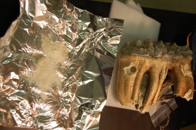
Sampling a mastodon molar from Boney Springs, Benton Co., MO. This was one of the first specimens we sampled. In later stages of the project we were much more “surgical” in our sampling.

We are also always interested in possible contamination. The amount of 14C in an organism is very small—and only gets smaller as it decays. When things are buried in the ground they are subject to all kinds of biological and geological processes. They are eaten by bacteria and mold. Roots and worms burrow into the outer surface. Water percolating through the soil can leave trace amounts of Carbon-rich minerals on the surface. So all of these things must be removed before we measure the amount of 14C in a sample.  When we date a bone, we want the date to reflect the time that the animal was alive—not all of the things that happened to it after it was buried. The “inorganic” or mineral component of bone (the part that gives bone its strength) is highly susceptible to this sort of contamination so we usually remove it and focus on the “organic” component—a mix of proteins, lipids, amino acids, and other goo that would have been present in the animal when it was alive. In the last decade or so we’ve gotten much better at dating bones. We pay close attention to the amounts of carbon and nitrogen in our samples to be sure that they are within the range of bones. If they fall outside of that range, it is possible they have been contaminated by post-depositional processes, or even the chemicals we use to stabilize and prepare specimens! The ability to measure very small samples also means we can isolate specific compounds from the bone itself, whether they be individual amino acids or short lengths of protein chains.

So what happens when you start dating lots of individual events? How do you make sense of broader spatial and chronological patterns? For the M-cubed project, we are dealing with just such a dataset. We’ve amassed a small mountain of data on where mammoths and mastodons were recovered, what they looked like, and importantly, how old they are. In collaboration with Greg Hodgins at the U of Az AMS lab, our dataset has increased to 96 reliable dates on mammoth and mastodon bones and teeth, spanning the last 50,000 years (some are even older). Although not as robust as the samples that modern ecologists amass by observing modern animals, this is a really decent dataset, and a far cry from the 17 well-dated sites that we had before starting the project.  Our intent is to tighten up our estimates of when these species went in extinct in the Midwest—so there are some bits of this dataset that help us understand these extinctions in more detail.

When is the youngest not the youngest, and how do we date something that isn’t there?

First, we can look at the youngest dates on mammoths (13,260 cal BP) and mastodons (12,710 cal BP). This is the traditional way of dealing with extinctions and makes intuitive sense. The youngest date on an animal is solid, concrete evidence that those animals were still around when this particular individual was alive. However, is it the only way of dating an extinction? After all, the odds of actually dating the last living individual of a species are pretty slim, a statistical improbability at best. Can we do better? Can we use the rest of our dataset to 1) get a better estimate on the actual age of extinction and 2) understand a bit more about how these animals went extinct?

The real challenge about putting a date (with error bars) on the extinction of Ice Age megafauna is that you can’t date what isn’t there. In other words, with more samples and wider coverage, we might capture younger and younger specimens, but the odds of getting that last mastodon standing are still really small. Unlike a rock stratum, we can’t constrain the date by the next youngest layer, so the error in our estimates will remain fairly large. But larger numbers of dates do help. And with a larger sample size, we can get a better idea of whether we are picking up the last dribbles, or whether we’re missing the last elephant standing in the corner of the room.

Rationale for calculation of extinction boundaries. If dates taper-off as extinction approaches, then then extinction envelope is broad. If there are many dates leading up to extinction, then envelope is narrow.

Stacey Lengyel, our chronology-specialist on this project, uses sophisticated statistics and modeling to estimate the error in our window of extinction (see Oxcal 4.2; calibration and Bayesian Modeling software). Take mastodons for example. Before we started the project we had 35 dates from 16 localities. Although the terminal age was 10,055+/-40 14C BP (aside: a date we could not replicate), the estimated error for the actual extinction window was fairly large 11,810-9380 cal BP. With the addition of 96 new dates (from 67 sites, with a few samples still pending) to the mix, the estimate of the extinction window narrowed drastically (12,500-12,780 cal BP). Part of the reason for this is that we increased the sample size of dated mastodons in the last few centuries prior to actual extinction.  We have more dated animals in the years leading up to that terminal date, which suggests if mastodons are around, then they are present in high enough numbers that we will sample them. It also means that—barring any massive changes in the region-wide preservation of these animals—the absence of dated mastodons AFTER this terminal date is “real” and not simply a function of poor sampling.

It’s a numbers game, and with more dates, we are on more solid footing when we attempt to order events in time. There are a whole slew of ideas about why these animals went extinct, and chronological contemporaneity is an important component of more than a few. Why is all of this important? Doesn’t it seem like we’re splitting hairs? What’s a few hundred years among friends? At the time these animals went extinct, there were lots of things going on. The first widespread evidence of a North American human presence, the Clovis period, dates from 13,200 to 12,800 years ago. There is a global return to glacial conditions called the Younger Dryas that begins ~12,800 years ago. Other species also went extinct at roughly the same time–but were they truly contemporary extinctions (yes, the verdict is still out on this)? We need maximum chronological resolution to establish an order of events. At the moment, it looks like mammoths and mastodons survived the Clovis period in the Midwest, becoming extinct at the beginning of the Younger Dryas. But before you think  “that settles it”, it is worth considering that most of our midwestern climate indicators (i.e., a network of lakes skirting the central and southern Great Lakes) suggest this climate shift was very gradual–at least at a regional scale. It was nowhere near drastic enough to unambiguously finger climate-change as the cause of the terminal Pleistocene extinctions.  For this, we’ll need other, complementary datasets on animal ecology, as well as region-specific information on human presence and environmental changes.  More on that in posts to come.